Poisson Process
Poisson Process simulation in R.
Definición:
Sean \(T_1\), \(T_2\), …, \(T_n\) v.a.i.i.d con distribución exponencial de parámetro \(\lambda\), : \(\mathcal{E}xp(\lambda)\). : \(\mathcal{W}_0=0\), \(\mathcal{W}_n=T_1, T_2, ..., T_n\) para \(n\geq 1\). Definimos el proceso Poisson de parámetro o intensidad \(\lambda\) por
$$\begin{equation}
 N(t)  =  máx \{n\geq 1, \  \ \mathcal{W}_n = T_1 + T_2 + ...+ T_n \leq t\}
 \end{equation}$$
Las variables aleatorias \(T_n\) representan los intervalos de tiempo entre eventos sucesivos, y \(\mathcal{W}_n = T_1, T_2, ..., T_n\) representa el instante en el que ocurre el n-ésimo evento, y \(N(t)\) es el número de eventos que han ocurrido hasta el instante \(t\).
Proposición:
La variable aleatoria \(N(t)\) tiene distribución Poisson con parámetro \((\lambda t)\), es decir, para cualquier \(t>0\), y para \(n=0, 1, ...\)
$$\begin{equation}
 P(N(t) = n) =  e^{-\lambda t} \frac{(\lambda t)^n}{n!}
 \end{equation}$$
Su valor esperado, y varianza son
$$E[N(t)] = \lambda t$$
$$Var(N(t)) = \lambda t$$
#   Reading packages
library("ggplot2")
library("dplyr")
library("plotly")
library("ggthemes")
library("tidyr")
library("stringr")
# Función para simular una trajectoria del proceso Poisson homogéneo
sim.one.PoissonProcess <- function(run, tmax, lambda){
  w <- c()
  w[1] <- 0
  i <- 2
  while(w[i-1] < tmax){
    #i <- i + 1
    Ti <- rexp(1, lambda)
    #print(Ti)
    if(w[i-1] +  Ti < tmax){
      w[i] <- w[i-1] +  Ti
    }else{
      break
    }
    i <- i + 1
  }
  df <- data.frame('runs' = rep(run, length(w)),
                   'n' = 0:(length(w)-1),
                   't' = w)
  return(df)
}

# Función para simular n trajectorias del proceso Poisson homogéneo
sim.PoissonProcess <- function(n.runs, tmax, lambda){
  for(i in 1:n.runs){
    if(i == 1){
      df_1 <- sim.one.PoissonProcess(run=i, tmax, lambda)
    }else{
      df_i <- sim.one.PoissonProcess(run=i, tmax, lambda)
      df_1 <- rbind(df_1, df_i)
    }

  }
  return(df_1)
}
Ejemplo 1: Una trayectoria del proceso Poisson
# Example :
n.runs <- 1 # número de trayectorias del proceso
tmax <- 500    # t máximo
lambda <- 0.2  # parámetro

# Simulación
sim.PP <- sim.PoissonProcess(n.runs, tmax, lambda)

# Media y varianza
moments_pp <- data.frame('t'=c(0:tmax),'lambda'=lambda) %>%
  mutate('mean' = t*lambda,
          'sd_inf' = mean - 2*sqrt(t*lambda),
          'sd_sup' = mean + 2*sqrt(t*lambda))
head(sim.PP)
##   runs n         t
## 1    1 0  0.000000
## 2    1 1  6.509327
## 3    1 2  8.934217
## 4    1 3 13.989072
## 5    1 4 14.494091
## 6    1 5 14.790950
# Gráfico del proceso Poisson
options(repr.plot.width=16, repr.plot.height=8)
p1 <- ggplot(sim.PP, mapping=aes(x=t, y=n, color = runs)) +
  geom_step(sim.PP, mapping=aes(x=t, y=n, group = runs), alpha = 0.25, col='black') +
  geom_step(moments_pp, mapping=aes(x=t,y=mean),col='red',size=0.7, alpha=0.5) +
  geom_step(moments_pp, mapping=aes(x=t,y=sd_sup),col='blue',size=0.7,linetype = "dashed") +
  geom_step(moments_pp, mapping=aes(x=t,y=sd_inf),col='blue',size=0.7,linetype = "dashed") +
  labs( title = paste(n.runs, "Trajectorias del proceso Poisson con lambda ", lambda)) +
  theme(legend.position = "none") +
  scale_colour_grey(start = 0.2,end = 0.8) +
  coord_cartesian(xlim = c(0, tmax))
p1

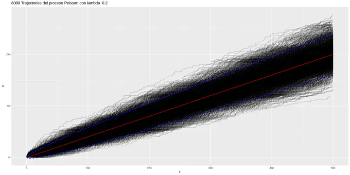
Ejemplo 2: Ocho mil trayectorias del proceso Poisson
# Example :
n.runs <- 8000 # número de trayectorias del proceso
tmax <- 500    # t máximo
lambda <- 0.2  # parámetro

# Simulación
sim.PP <- sim.PoissonProcess(n.runs, tmax, lambda)

# Media y varianza
moments_pp <- data.frame('t'=c(0:tmax),'lambda'=lambda) %>%
  mutate('mean' = t*lambda,
          'sd_inf' = mean - 2*sqrt(t*lambda),
          'sd_sup' = mean + 2*sqrt(t*lambda))
# Gráfico del proceso Poisson
options(repr.plot.width=16, repr.plot.height=8)
p1 <- ggplot(sim.PP, mapping=aes(x=t, y=n, color = runs)) +
  geom_step(sim.PP, mapping=aes(x=t, y=n, group = runs), alpha = 0.25, col='black') +
  geom_step(moments_pp, mapping=aes(x=t,y=mean),col='red',size=0.7, alpha=0.5) +
  geom_step(moments_pp, mapping=aes(x=t,y=sd_sup),col='blue',size=0.7,linetype = "dashed") +
  geom_step(moments_pp, mapping=aes(x=t,y=sd_inf),col='blue',size=0.7,linetype = "dashed") +
  labs( title = paste(n.runs, "Trajectorias del proceso Poisson con lambda ", lambda)) +
  theme(legend.position = "none") +
  scale_colour_grey(start = 0.2,end = 0.8) +
  coord_cartesian(xlim = c(0, tmax))
p1

Valor esperado y varianza de \(N(t)\):
$$E[N(t)] = \lambda t $$ $$Var(N(t)) = \lambda t $$
Para este ejemplo con \(t=50\) y \(\lambda = 0.2\):
$$E[N(t)] = 0.2(50) = 10$$
$$Var(N(t)) = 0.2(50) = 10$$
# Verificación mediante simulación para t=50
sim.PP %>% filter(t<=50) %>% group_by(runs) %>% summarise(Nt=max(n)) %>% summarise(mean=mean(Nt), var=var(Nt))
## # A tibble: 1 × 2
##    mean   var
##   <dbl> <dbl>
## 1  10.1  10.0
Covarianza
Para un proceso Poisson con parámetro lambda \(\lambda\), y \(s<t\) la covarianza entre \(N(s)\) y \(N(t)\) es
$$\begin{equation}
 Cov(N(s), N(t))  =  \lambda s
 \end{equation}$$
Ejemplo:
Obtener:
1.- \(Cov(N(5), N(6))\)
2.- \(Cov(N(10), N(100))\)
Solución teórica:
1.- \(Cov(N(5), N(6))= \lambda s = (0.2)(5)= 1\)
2.- \(Cov(N(100), N(40))= \lambda s = (0.2)(40)= 8\)
Simulación:
# Solución $Cov(N(5), N(6))$

# Obtenemos N(5)
N_5 <- sim.PP %>% filter(t<=5) %>% group_by(runs) %>% summarise(Nt=max(n))%>% select(Nt) %>% pull()
# Obtenemos N(6)
N_6 <- sim.PP %>% filter(t<=6) %>% group_by(runs) %>% summarise(Nt=max(n))%>% select(Nt) %>% pull()

# Calculamos la covarianza muestreal entre N(5) y N(6))
round(cov(N_5, N_6),2)
## [1] 1
# Solución Cov(N(100), N(40))

# N(100)
N_100 <- sim.PP %>% filter(t<=100) %>% group_by(runs) %>% summarise(Nt=max(n))%>% select(Nt) %>% pull()
# N(40)
N_40 <- sim.PP %>% filter(t<=40) %>% group_by(runs) %>% summarise(Nt=max(n))%>% select(Nt) %>% pull()

# Calculamos la covarianza muestreal entre N(100) y N(40))
round(cov(N_100, N_40),2)
## [1] 7.89
Julio Cesar Martinez
My research interests include statistics, stochastic processes and data science.