Pearson Random Walk
Pearson Random Walk simulation in Python.
import pandas as pd
import numpy as np
from numpy.random import uniform
import matplotlib.pyplot as plt
import seaborn as sns
sns.set()
Origen
Sea $$ \overrightarrow{R}_n = \overrightarrow{r}_1 + \overrightarrow{r}_2 + … + \overrightarrow{r}_n $$
donde
\begin{equation}
 \overrightarrow{R}_x = l \sum_{i=1}^{n} cos(\theta_i)\\
 \overrightarrow{R}_y = l \sum_{i=1}^{n} sen(\theta_i)
 \end{equation}
$$|R_n| = \sqrt{\overrightarrow{R}_x + \overrightarrow{R}_y} $$
# Pearson Random Walk function
def PearsonRandomWalk(nsteps, l=1):
  rx = [0]*(nsteps+1)
  ry = [0]*(nsteps+1)
  for i in range(1, nsteps+1):
    theta = uniform(low=0, high=2*np.pi, size=1)[0]
    rx[i] = l*np.cos(theta)
    ry[i] = l*np.sin(theta)
  rx = np.array(rx)
  ry = np.array(ry)
  Rx = rx.cumsum()
  Ry = ry.cumsum()
  R2 = Rx**2 + Ry**2
  R = np.sqrt(R2)

  return rx, ry, Rx, Ry, R2, R
nsteps = 5000
npaths = 5000
# multiple paths
rxs, rys, Rxs, Rys, R2s, Rs = [], [], [], [], [], []
# loop
for i in range(npaths):
  rx, ry, Rx, Ry, R2, R = PearsonRandomWalk(nsteps)
  rxs.append(rx)
  rys.append(ry)
  Rxs.append(Rx)
  Rys.append(Ry)
  R2s.append(R2)
  Rs.append(R)
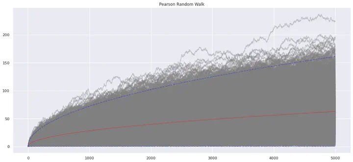
Caminata Aleatoria de Pearson
x = np.array([*range(nsteps+1)])
# media y varianza de la distribución Rayleigh
mean = np.sqrt(x/2)*np.sqrt(np.pi/2)
variance = ((x/2))*((4-np.pi)/2)
# gráfico
plt.figure(figsize=(18,8))
for r in Rs:
  plt.plot(x, r, '-', color='grey', alpha=0.4)
plt.plot(x, mean, '-', color='red', alpha=0.4)
plt.plot(x, mean + 3*np.sqrt(variance), '--', color='blue', alpha=0.4)
plt.plot(x, [0]*len(x), '--', color='blue', alpha=0.4)
plt.title('Pearson Random Walk')
plt.show()

Veamos el promedio de las trayetorias con respecto a \(t\).
x = np.array([*range(nsteps+1)])
plt.figure(figsize=(18,8))
plt.plot(np.array(Rs).mean(axis=0) , '.', color='grey', alpha=0.9, label='Promedio')
plt.plot(x, np.sqrt(x/2)*np.sqrt(np.pi/2), '-', color='blue', alpha=0.4, label='Valor esperado teórico')
plt.title('Pearson Random Walk')
plt.legend()
plt.show()

Distribución de \(\overrightarrow{R}_n\)
Rn = [r[nsteps] for r in Rs]
plt.figure(figsize=(16,7))
sns.kdeplot(Rn, color='red')
plt.hist(Rn, bins=40, density=True)
plt.title('Distribución de $R_n$')
plt.show()

Distribución de \(\overrightarrow{R}_x\)
$$\overrightarrow{R}_x \sim N(0, n/2)$$
Rx = [rx[nsteps] for rx in Rxs]
plt.figure(figsize=(16,7))
sns.kdeplot(Rx, color='red')
plt.hist(Rx, bins=50, density=True)
plt.title('Distribución de $R_x$')
plt.show()

Distribución de \(\overrightarrow{R}_y\)
$$\overrightarrow{R}_y \sim N(0, n/2)$$
Ry = [ry[nsteps] for ry in Rys]
plt.figure(figsize=(16,7))
sns.kdeplot(Ry, color='red')
plt.hist(Ry, bins=50, density=True)
plt.title('Distribución de $R_y$')
plt.show()

Distribución de \(R_n^2\)
Sea \(W= R_n^2 = \overrightarrow{R}_x^2 + \overrightarrow{R}_y^2\), entonces la distribución viene dada por
\begin{equation}
 f_W(w) = \frac{1}{n} \exp\{- \frac{w}{n}\}, \ \ \ w>0
 \end{equation}
R2 = [r2[nsteps] for r2 in R2s]
plt.figure(figsize=(16,7))
plt.hist(R2, bins=50, density=True)
plt.title('Distribución de $R_n^2$')
plt.show()

Trayectoria del Caminante
plt.figure(figsize=(14,10))
plt.plot(Rxs[1], Rys[1], 'o', color='blue', markersize=3)
plt.plot(Rxs[1], Rys[1], color='black', linewidth=0.8)
plt.title('Pearson Random Walk')
plt.xlabel('Time')
#mplcyberpunk.add_glow_effects()
plt.show()

Julio Cesar Martinez
My research interests include statistics, stochastic processes and data science.